rayrender

Overview

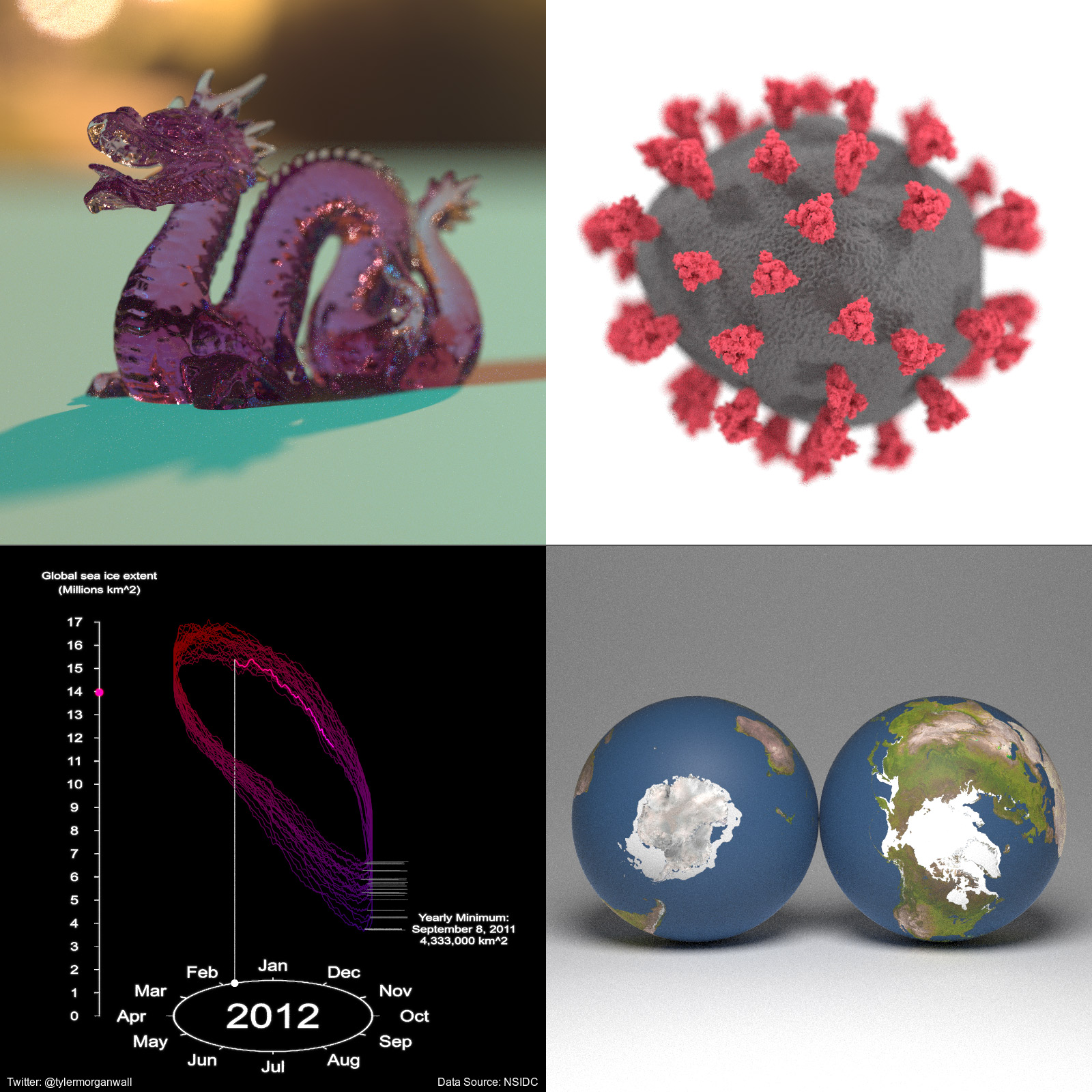
rayrender is an open source R package for raytracing scenes in created in R. This package provides a tidy R interface to a fast pathtracer written in C++ to render scenes built out of an array of primitives and meshes. rayrender builds scenes using a pipeable iterative interface, and supports diffuse, metallic, dielectric (glass), glossy, microfacet, light emitting materials, as well as procedural and user-specified image/roughness/bump/normal textures and HDR environment lighting. rayrender includes multicore support (with progress bars) via RcppThread, random number generation via the PCG RNG, OBJ/PLY support, and denoising support with Intel Open Image Denoise (OIDN).

Browse the documentation and see more examples at the website (if you aren’t already there):

rayrender.net

Installation

# To install the latest version from Github:
# install.packages("devtools")
devtools::install_github("tylermorganwall/rayrender")

Optional: denoising with Intel Open Image Denoise (OIDN)

rayrender can use Intel Open Image Denoise to denoise rendered images when OIDN is available on your system. If OIDN is not found, rayrender will still work, just without denoising support.

To get denoising support, you need to install OIDN. You can download the official binaries from Intel and set the OIDN_PATH argument in your .Renviron file with the following command line instructions:

macOS

# Download the appropriate binary for your architecture
curl -LO https://github.com/OpenImageDenoise/oidn/releases/download/v2.3.1/oidn-2.3.1.x86_64.macos.tar.gz
# or for Apple Silicon
curl -LO https://github.com/OpenImageDenoise/oidn/releases/download/v2.3.1/oidn-2.3.1.arm64.macos.tar.gz

# Extract the archive
tar -xvzf oidn-2.3.1.x86_64.macos.tar.gz
# or for Apple Silicon
tar -xvzf oidn-2.3.1.arm64.macos.tar.gz

# Set OIDN_PATH in your .Renviron file to the extracted directory
echo "OIDN_PATH=/path/to/extracted/oidn" >> ~/.Renviron

linux

# Download the binary
curl -LO https://github.com/OpenImageDenoise/oidn/releases/download/v2.3.1/oidn-2.3.1.x86_64.linux.tar.gz

# Extract the archive
tar -xvzf oidn-2.3.1.x86_64.linux.tar.gz

# Set OIDN_PATH in your .Renviron file to the extracted directory
echo "OIDN_PATH=/path/to/extracted/oidn" >> ~/.Renviron

Windows (Rtools45)

Windows is slightly trickier and requires Rtools45. The steps are:

1. Install make and ninja via RTools.
2. Install ISPC (Intel SPMD Program Compiler).
3. Download the OIDN source repository.
4. Compile and install OIDN, and point rayrender to it via OIDN_PATH.

OIDN_PATH should point to a directory that contains include/OpenImageDenoise and lib (or lib64) with the OIDN libraries.

Install prerequisites

1. Install Rtools45 https://cran.r-project.org/bin/windows/Rtools/
2. Open the “Rtools45 MinGW UCRT64” shell (ucrt64) in RTools45.
3. Inside that shell, install the build tools (including make, ninja, cmake, git, and ispc) via pacman:

pacman -Sy --needed \
    mingw-w64-ucrt-x86_64-make \
    mingw-w64-ucrt-x86_64-ninja \
    mingw-w64-ucrt-x86_64-cmake \
    mingw-w64-ucrt-x86_64-ispc

4. Make sure the Rtools static-posix toolchain and the MinGW binaries are on PATH (this mirrors the setup used to build OIDN):

export PATH="/c/rtools45/x86_64-w64-mingw32.static.posix/bin:/mingw64/bin:${PATH}"

5. Verify the toolchain:

gcc --version
g++ --version
make --version
ninja --version
cmake --version
ispc --version

5. Confirm ISPC is available:

ispc --version

Build and install OIDN from source (CPU-only)

All of the following commands are run from the Rtools45 ucrt64 shell:

# Download the OIDN source
git clone --recursive https://github.com/RenderKit/oidn.git
cd oidn

# Create a separate build directory
mkdir build-cpu-static
cd build-cpu-static

# Choose an install prefix; use a simple path without spaces
# This will become C:/local/oidn-static on Windows
OIDN_PREFIX="C:/local/oidn-static"

# Configure OIDN with the Rtools static-posix toolchain, CPU-only, static lib
# Update with your rtools45 path.
cmake \
  -G "Ninja" \
  -DCMAKE_BUILD_TYPE=Release \
  -DCMAKE_C_COMPILER="/path/to/rtools45/x86_64-w64-mingw32.static.posix/bin/gcc.exe" \
  -DCMAKE_CXX_COMPILER="/path/to/rtools45/x86_64-w64-mingw32.static.posix/bin/g++.exe" \
  -DOIDN_STATIC_LIB=ON \
  -DOIDN_DEVICE_CPU=ON \
  -DOIDN_DEVICE_SYCL=OFF \
  -DOIDN_DEVICE_CUDA=OFF \
  -DOIDN_DEVICE_HIP=OFF \
  -DOIDN_DEVICE_METAL=OFF \
  -DOIDN_APPS=OFF \
  -DISPC_EXECUTABLE="$(command -v ispc)" \
  -DTBB_DIR="/path/to/rtools45/x86_64-w64-mingw32.static.posix/lib/cmake/TBB" \
  -DCMAKE_INSTALL_PREFIX="${OIDN_PREFIX}" \
  ..

If CMake cannot find TBB in Rtools automatically, add a hint such as:

-DTBB_ROOT=/path/to/rtools45/x86_64-w64-mingw32.static.posix

(adjust the path for your actual Rtools45 install) to the cmake command above.

Then build and install:

ninja
ninja install

After installation you should have, for example:

C:/local/oidn/include/OpenImageDenoise/oidn.h
C:/local/oidn/lib/libOpenImageDenoise.a   (and related libs)

Tell R where OIDN lives

In a regular Windows shell or PowerShell, add to your user .Renviron:

echo 'OIDN_PATH=C:/local/oidn' >> "$HOME/.Renviron"

or edit the file and add the above manually with devtools::edit_r_environ().

Restart R (or your IDE), then reinstall rayrender from source:

devtools::install_github("tylermorganwall/rayrender", force = TRUE)

After this, rayrender should detect OIDN during configure and enable denoising support on Windows.

Usage

We’ll first start by rendering a simple scene consisting of the ground, a sphere, and the included R.obj file. The location of the R.obj file can be accessed by calling the function r_obj(). First adding the ground using the render_ground() function. This renders an extremely large sphere that (at our scene’s scale) functions as a flat surface. We also add a simple blue sphere to the scene.

library(rayrender)

scene = generate_ground(material=diffuse(checkercolor="grey20")) %>%
  add_object(sphere(y=0.2,material=glossy(color="#2b6eff",reflectance=0.05))) 
render_scene(scene, parallel = TRUE, width = 800, height = 800, samples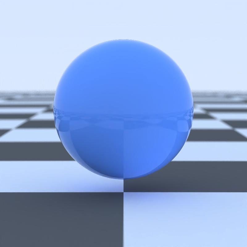 = 64)

By default, a scene without any lights includes a blue sky. We can turn this off either by setting ambient_light = FALSE, or by adding a light to our scene. We will add an emissive sphere above and behind our camera.

scene = generate_ground(material=diffuse(checkercolor="grey20")) %>%
  add_object(sphere(y=0.2,material=glossy(color="#2b6eff",reflectance=0.05))) %>%
  add_object(sphere(y=10,z=1,radius=4,material=light(intensity=4))) %>%
  add_object(sphere(z=15,material=light(intensity=70)))
render_scene(scene, parallel = TRUE, width = 800, height = 800, samples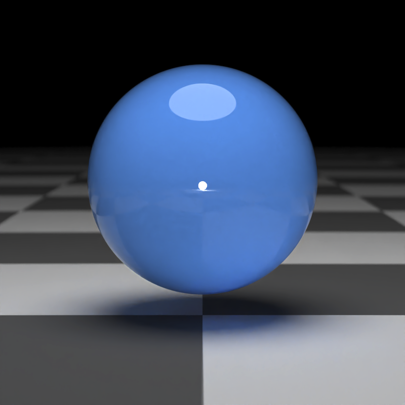 = 64)

Now we’ll add the (included) R .obj file into the scene, using the obj_model() function. We will scale it down slightly using the scale_obj argument, and then embed it on the surface of the ball.

scene = generate_ground(material=diffuse(checkercolor="grey20")) %>%
  add_object(sphere(y=0.2,material=glossy(color="#2b6eff",reflectance=0.05))) %>%
  add_object(obj_model(r_obj(simple_r = TRUE),
                       z=1,y=-0.05,scale_obj=0.45,material=diffuse())) %>%
  add_object(sphere(y=10,z=1,radius=4,material=light(intensity=4))) %>%
  add_object(sphere(z=15,material=light(intensity=70)))
render_scene(scene, parallel = TRUE, width = 800, height = 800, samples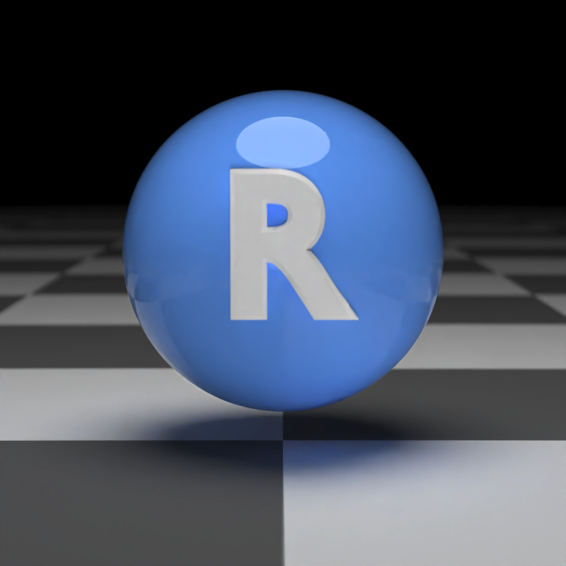 = 64)

Here we’ll render a grid of different viewpoints.

filename = tempfile()
image1 = render_scene(scene, parallel = TRUE, width = 400, height = 400, 
             lookfrom = c(7,1,7), samples = 64, return_raw_array = TRUE)
image2 = render_scene(scene, parallel = TRUE, width = 400, height = 400, 
             lookfrom = c(0,7,7), samples = 64, return_raw_array = TRUE)
image3 = render_scene(scene, parallel = TRUE, width = 400, height = 400, 
             lookfrom = c(-7,0,-7), samples = 64, return_raw_array = TRUE)
image4 = render_scene(scene, parallel = TRUE, width = 400, height = 400, 
             lookfrom = c(-7,7,7), samples = 64, return_raw_array = TRUE)
rayimage::plot_image_grid(list(image1,image2,image3,image4), dim = c(2,2))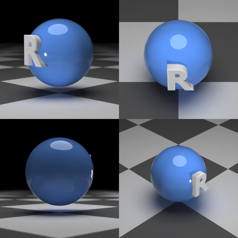

Here’s another example: We start by generating an empty Cornell box and rendering it with render_scene(). Setting parallel = TRUE will utilize all available cores on your machine. The lookat, lookfrom, aperture, and fov arguments control the camera, and the samples argument controls how many samples to take at each pixel. Higher sample counts result in a less noisy image.

scene = generate_cornell()
render_scene(scene, lookfrom=c(278,278,-800),lookat = c(278,278,0), aperture=0, fov=40, samples = 64,
             ambient_light=FALSE, parallel=TRUE, width=800, height=800)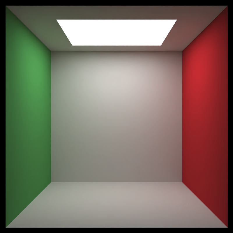

Here we add a metal ellipsoid, a checkered purple cube, a colored glass sphere, a pig, and plaster the walls with the iris dataset using textures applied to rectangles. We first write the textures out to a temporary filename, and then read the image back in using the png::readPNG() function. We then pass this to the image argument in the diffuse material, which applies it as a texture.

tempfileplot = tempfile()
png(filename=tempfileplot,height=1600,width=1600)
plot(iris$Petal.Length,iris$Sepal.Width,col=iris$Species,pch=18,cex=12)
dev.off()

## quartz_off_screen 
##                 2

image_array = png::readPNG(tempfileplot)

generate_cornell() %>%
  add_object(ellipsoid(x=555/2,y=100,z=555/2,a=50,b=100,c=50, material = metal(color="lightblue"))) %>%
  add_object(cube(x=100,y=130/2,z=200,xwidth = 130,ywidth=130,zwidth = 130,
                  material=diffuse(checkercolor="purple", checkerperiod = 30),angle=c(0,10,0))) %>%
  add_object(pig(x=100,y=190,z=200,scale=40,angle=c(0,30,0))) %>%
  add_object(sphere(x=420,y=555/8,z=100,radius=555/8,
                    material = dielectric(color="orange"))) %>%
  add_object(yz_rect(x=0.01,y=300,z=555/2,zwidth=400,ywidth=400,
                     material = diffuse(image_texture = image_array))) %>%
  add_object(yz_rect(x=555/2,y=300,z=555-0.01,zwidth=400,ywidth=400,
                     material = diffuse(image_texture = image_array),angle=c(0,90,0))) %>%
  add_object(yz_rect(x=555-0.01,y=300,z=555/2,zwidth=400,ywidth=400,
                     material = diffuse(image_texture = image_array),angle=c(0,180,0))) %>%
  render_scene(lookfrom=c(278,278,-800),lookat = c(278,278,0), aperture=0, fov=40,  samples = 64,
             ambient_light=FALSE, parallel=TRUE, width=800, height=800)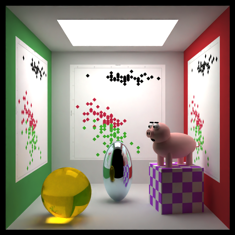

Rayrender also has an interface to create objects using constructive solid geometry, with a wide variety of primitives and operations.

generate_ground(material=diffuse(checkercolor="grey20")) %>%
  add_object(csg_object(csg_combine(
    csg_combine(
      csg_box(),
      csg_sphere(radius=0.707),
      operation="intersection"),
    csg_group(list(csg_cylinder(start=c(-1,0,0), end=c(1,0,0), radius=0.4),
                   csg_cylinder(start=c(0,-1,0), end=c(0,1,0), radius=0.4),
                   csg_cylinder(start=c(0,0,-1), end=c(0,0,1), radius=0.4))),
    operation="subtract"),
    material=glossy(color="red"))) %>%
  add_object(csg_object(csg_translate(csg_combine(
    csg_onion(csg_onion(csg_onion(csg_sphere(radius=0.3), 0.2), 0.1),0.05),
    csg_box(y=1,width=c(10,2,10)), operation = "subtract"), x=1.3),
    material=glossy(color="purple"))) %>%
  add_object(csg_object(csg_combine(
     csg_sphere(x=-1.2,z=-0.3, y=0.5,radius = 0.4),
     csg_sphere(x=-1.4,z=0.4, radius = 0.4), operation="blend", radius=0.5),
     material=glossy(color="dodgerblue4"))) %>%
  add_object(sphere(y=5,x=3,radius=1,material=light(intensity=30))) %>%
  render_scene(clamp_value=10, fov=20,lookfrom=c(5,5,10),samples=64,width=800,height=800)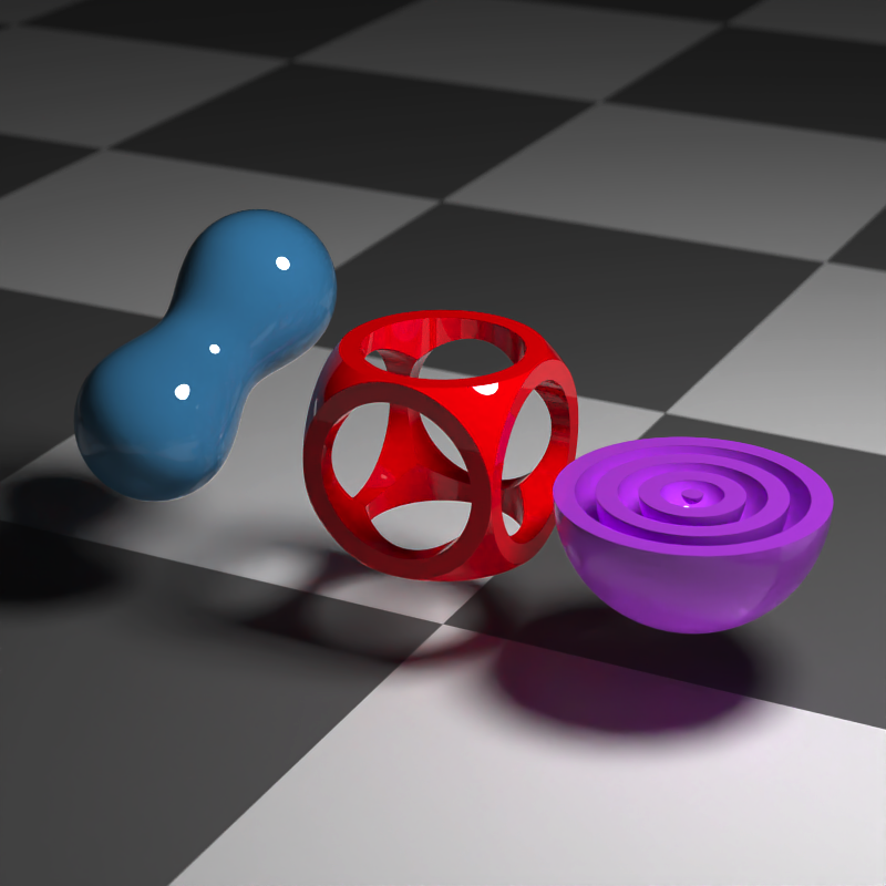

We can also use the path() element to draw 3D paths. Here, we render the Lorenz attractor:

library(deSolve)
parameters = c(s = 10, r = 28, b = 8/3)
state = c(X = 1, Y = 0, Z = 1)

Lorenz = function(t, state, parameters) {
  with(as.list(c(state, parameters)), {
    dX = s * (Y - X)
    dY = X * (r - Z) - Y
    dZ = X * Y - b * Z
    list(c(dX, dY, dZ))
  })
}

times = seq(0, 50, by = 0.05)
vals = ode(y = state, times = times, func = Lorenz, parms = parameters)[,-1]

#scale and rearrange:
vals = vals[,c(1,3,2)]/20

generate_studio() %>% 
  add_object(path(points=vals,y=-0.6,width=0.01,material=diffuse(color="red"))) %>% 
  add_object(sphere(y=5,z=5,radius=0.5,material=light(intensity=200))) %>% 
  render_scene(samples=64,lookat=c(0,0.5,0),lookfrom=c(0,1,10),width = 800, height = 800, parallel=TRUE)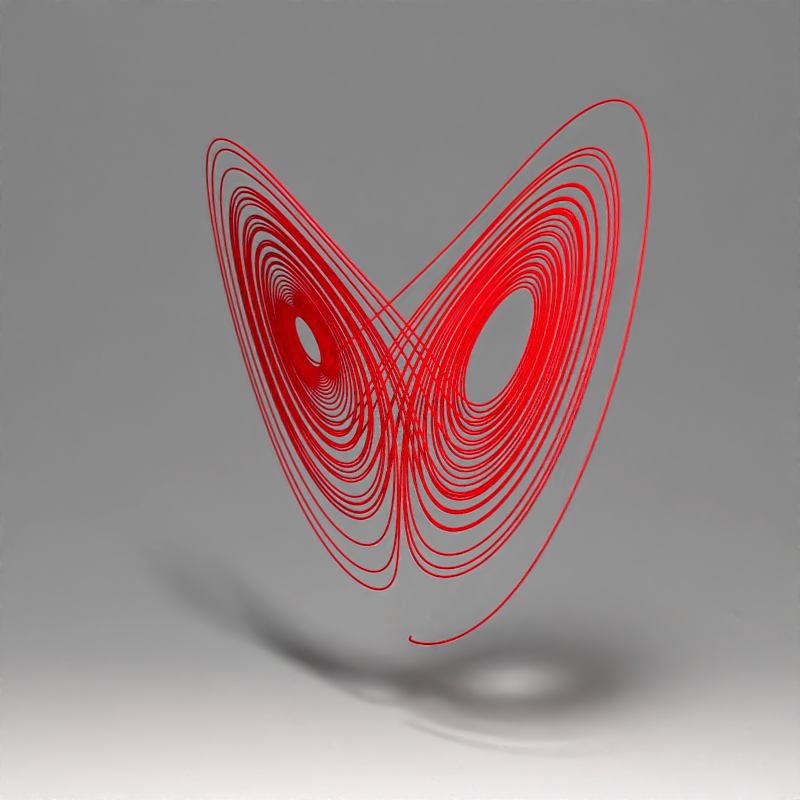

rayrender also supports an extruded path object that generates a variable width path with any non-intersecting simple polygon (including holes) as an input. You can vary the width, add twist, and change the shape of the polygon along the path’s length.

points = list(c(0,0,1),c(-0.5,0,-1),c(0,1,-1),c(1,0.5,0),c(0.6,0.3,1))
#Create star polygon
angles = seq(0,360,by=36)
xx = rev(c(rep(c(1,0.5),5),1) * sinpi(angles/180))
yy = rev(c(rep(c(1,0.5),5),1) * cospi(angles/180))
star_polygon = data.frame(x=xx,y=yy)

#Extrude a path using a star polygon
generate_studio(depth=-0.4) |>
  add_object(extruded_path(points = points, width=abs(cospi(seq(0,4,by=0.01)))/4,
                           polygon = star_polygon,
                           twists = 4,
                           breaks = 1000,
                           material=diffuse(color="purple"))) |>
  add_object(sphere(y=3,z=5,x=2,radius=1,material=light(intensity=15))) |>
  render_scene(lookat=c(0.3,0.5,1), 
               fov=12, width=800,height=800, 
               aperture=0.025, samples=64)

## Warning in mesh3d_model(mesh, x = x, y = y, z = z, override_material = TRUE, :
## material set as vertex color but no texture or bump map passed--ignoring mesh3d
## material.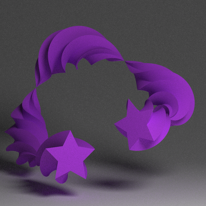

#Render a closed Mobius strip with 1.5 turns 
points = list(c(0,0,0),c(0.5,0.5,0),c(0,1,0),c(-0.5,0.5,0))
square_polygon = matrix(c(-1, -0.1, 0,
                           1, -0.1, 0,
                           1,  0.1, 0,
                          -1,  0.1, 0)/10, ncol=3,byrow = T)

generate_studio(depth=-0.2,
               material=diffuse(color = "dodgerblue4", checkercolor = "#002a61",
                                checkerperiod = 1)) |>
 add_object(extruded_path(points = points,  polygon=square_polygon, closed = TRUE,
                          linear_step = TRUE, twists = 1.5, breaks = 720, 
                          material = diffuse(noisecolor = "black", noise = 10, 
                                             noiseintensity = 10))) |>
 add_object(sphere(y=20,x=0,z=21,material=light(intensity = 1000))) |> 
 render_scene(lookat=c(0,0.5,0), fov=10, samples=64,
              width = 800, height=800)

## Warning in mesh3d_model(mesh, x = x, y = y, z = z, override_material = TRUE, :
## material set as vertex color but no texture or bump map passed--ignoring mesh3d
## material.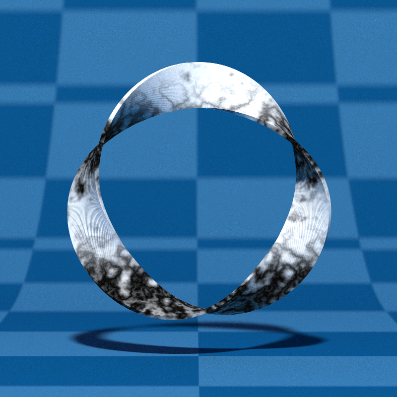

Finally, rayrender supports environment lighting with the environment_light argument. Pass a high dynamic range image (.hdr) or a low-dynamic range image (.jpg,.png) and the image will be used to light the scene (along with any other lights). Here’s an example using an HDR image of Venice at sunset (obtained for free from hdrihaven.com), also using the Oren-Nayar diffuse model with sigma = 90 for a more realistic diffuse surface. We also add an extruded polygon star, using the extruded_polygon object.

tempfilehdr = tempfile(fileext = ".hdr")
download.file("https://www.tylermw.com/data/venice_sunset_2k.hdr",tempfilehdr, mode="wb")
hollow_star = rbind(star_polygon, 0.8 * star_polygon)

generate_ground(material = diffuse(color="grey20", checkercolor = "grey50",sigma=90)) %>%
  add_object(sphere(material=microfacet(roughness = 0.2,
                                        eta=c(0.216,0.42833,1.3184), kappa=c(3.239,2.4599,1.8661)))) %>%
  add_object(obj_model(y=-1,x=-1.8,r_obj(simple_r = TRUE), 
                       angle=c(0,135,0),material = diffuse(sigma=90))) %>%
  add_object(pig(x=1.8,y=-1.2,scale=0.5,angle=c(0,90,0),diffuse_sigma = 90)) %>%
  add_object(extruded_polygon(hollow_star,top=-0.5,bottom=-1, z=-2,
                              holes = nrow(star_polygon),
                              material=diffuse(color="red",sigma=90))) %>%
  render_scene(parallel = TRUE, environment_light = tempfilehdr, width=800,height=800,
               fov=70,samples=64, aperture=0.1, sample_method = "sobol_blue",
               lookfrom=c(-0.9,1.2,-4.5),lookat=c(0,-1,0))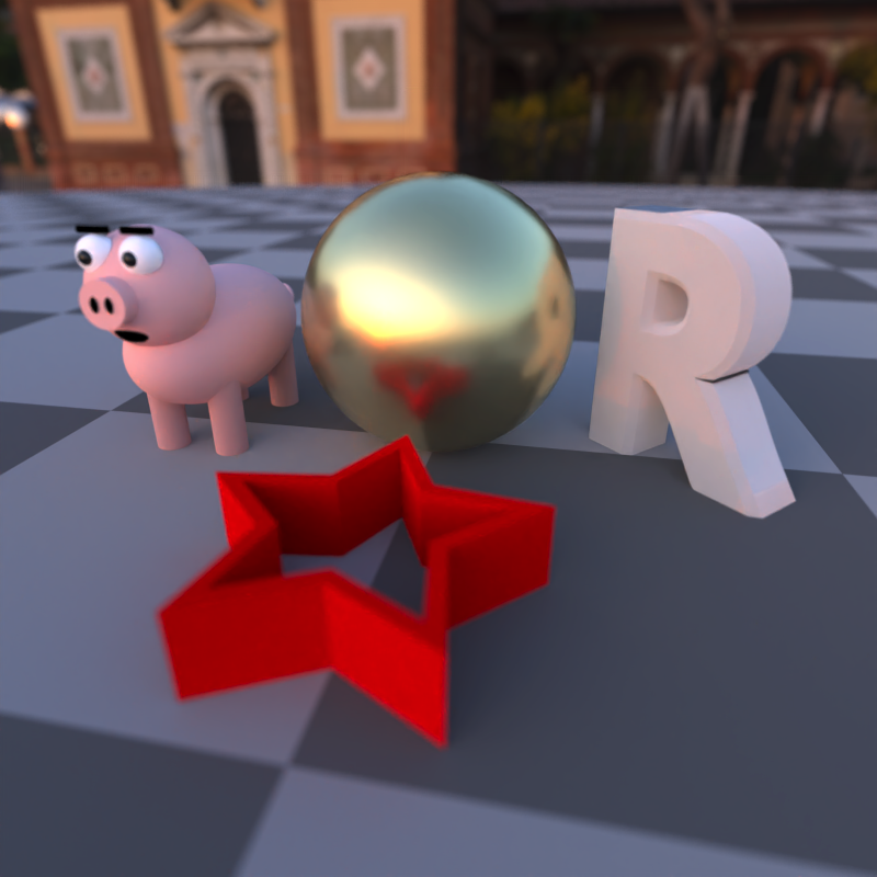

Acknowledgments

Thanks to Brodie Gaslam (@brodieG) for contributions to the extruded_polygon() function.